On Benchmarking MiniZinc and the LinkedIn Queens ProblemDRAFT
In Solving LinkedIn Queens using MiniZinc I wrote about how to solve the LinkedIn Queens problem using MiniZinc, and showed a single example. In Solving LinkedIn Queens with Haskell I saw that there is a large set of instances available, so it’s time to benchmark the different MiniZinc solvers.
The benchmarks test several different features, so first it’s worth going deeper into what MiniZinc actually is and how it works. In addition, we will talk about how to benchmark solvers and what the different values mean.
If you are in a hurry, the short answer is that since the existing available instances are quite small (up to size 11), most solvers will work more or less equally well. This also means that there mostly won’t be any important differences to show in behavior, as there could be with larger and harder instances. LinkedIn Queens is still quite an instructive example and will show how to think about MiniZinc performance.
Background: MiniZinc compilation and execution
Before the benchmarks will make sense, a better understanding of what MiniZinc is and does is needed.
MiniZinc compilation and FlatZinc
MiniZinc is a modeling language that is solver agnostic. The first step in solving a problem modeled with MiniZinc is for the system to read the model, the data file, and the settings for the intended solver. This is used to compile the model down to a lower-level format used by the solver called FlatZinc. The compiled FlatZinc format is essentially a list of all the variables and all the constraints in the problem.
When MiniZinc reads the line
include "globals.mzn";this reads the definition from the standard library supplied with a solver.
This library can define a constraint like all_different as some global constraint the solver supports,
or it can supply a decomposition into simpler constraints.
In this example, given an array array[N] of var N: x and the constraint all_different(x),
the standard decomposition would be x[1] != x[2] /\ x[1] != x[3] /\ ..., so just all the different not-equals constraints.
In FlatZinc, each constraint x[1] != x[2] would be represented by a pre-defined predicate int_ne(x[1], x[2]).
Example: A minimal instance
To see the difference between MiniZinc and FlatZinc, we will look at a minimal example. First recall the full model from the previous post, and now consider this minimal example puzzle.
n = 4;
Colors = {P, W, S, R};
board = [|P, P, P, P  |P, P, R, S  |R, R, R, W  |R, R, W, W  ||];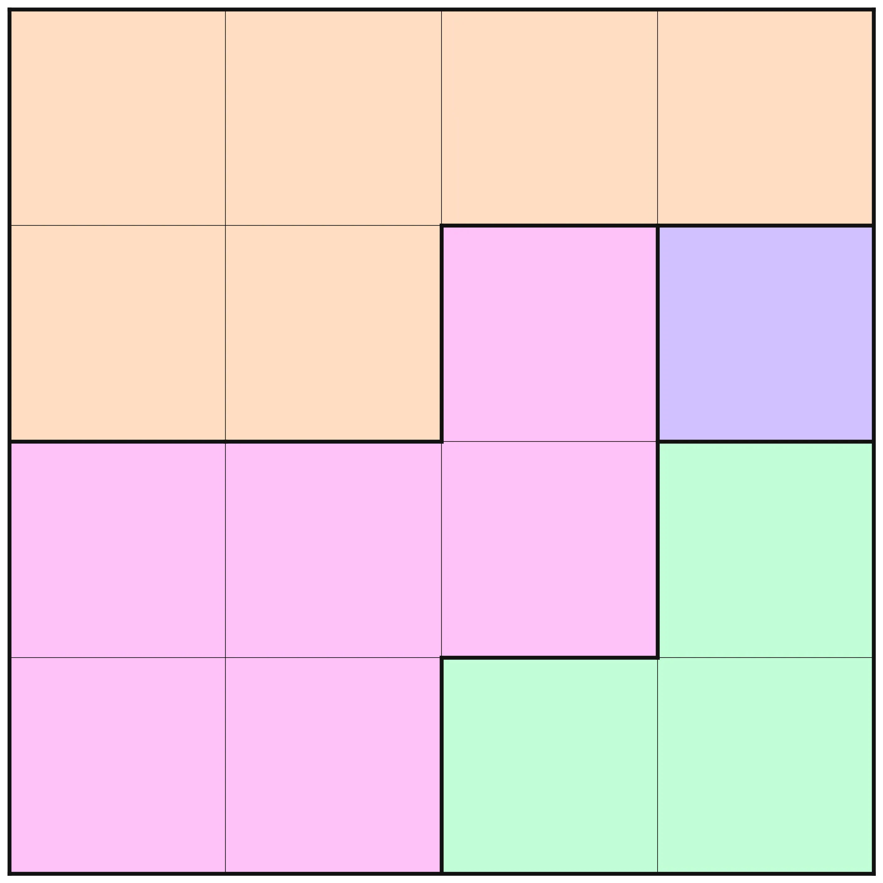
This can be compiled into a FlatZinc file for the Gecode solver using the following command.
$ minizinc --solver gecode -c linkedin-queens.mzn mini.dzn --fzn mini-gecode.fznThe file produced can be used as input to the fzn-gecode binary from the Gecode distribution, and the file looks like this.
predicate fzn_all_different_int(array [int] of var int: x);predicate gecode_int_element(var int: idx,int: idxoffset,array [int] of var int: x,var int: c);var 1..4: X_INTRODUCED_35_;var 1..4: X_INTRODUCED_36_;var 1..4: X_INTRODUCED_37_;var 1..4: X_INTRODUCED_38_;var -3..3: X_INTRODUCED_40_ ::var_is_introduced :: is_defined_var;var 2..3: X_INTRODUCED_41_ ::var_is_introduced :: is_defined_var;var -3..3: X_INTRODUCED_42_ ::var_is_introduced :: is_defined_var;var 2..3: X_INTRODUCED_43_ ::var_is_introduced :: is_defined_var;var -3..3: X_INTRODUCED_44_ ::var_is_introduced :: is_defined_var;var 2..3: X_INTRODUCED_45_ ::var_is_introduced :: is_defined_var;var 1..4: X_INTRODUCED_50_ ::var_is_introduced :: is_defined_var;var 2..4: X_INTRODUCED_52_ ::var_is_introduced :: is_defined_var;var 1..4: X_INTRODUCED_54_ ::var_is_introduced :: is_defined_var;array [1..4] of var int: queens:: output_array([1..4]) = [X_INTRODUCED_35_,X_INTRODUCED_36_,X_INTRODUCED_37_,X_INTRODUCED_38_];array [1..4] of var int: X_INTRODUCED_55_ ::var_is_introduced = [1,X_INTRODUCED_50_,X_INTRODUCED_52_,X_INTRODUCED_54_];constraint fzn_all_different_int(queens);constraint int_abs(X_INTRODUCED_40_,X_INTRODUCED_41_):: defines_var(X_INTRODUCED_41_);constraint int_abs(X_INTRODUCED_42_,X_INTRODUCED_43_):: defines_var(X_INTRODUCED_43_);constraint int_abs(X_INTRODUCED_44_,X_INTRODUCED_45_):: defines_var(X_INTRODUCED_45_);constraint gecode_int_element(X_INTRODUCED_35_,1,[1,1,1,1],1);constraint gecode_int_element(X_INTRODUCED_36_,1,[1,1,4,3],X_INTRODUCED_50_):: defines_var(X_INTRODUCED_50_);constraint gecode_int_element(X_INTRODUCED_37_,1,[4,4,4,2],X_INTRODUCED_52_):: defines_var(X_INTRODUCED_52_);constraint gecode_int_element(X_INTRODUCED_38_,1,[1,4,2,2],X_INTRODUCED_54_):: defines_var(X_INTRODUCED_54_);constraint fzn_all_different_int(X_INTRODUCED_55_);constraint int_lin_eq([1,-1,-1],[X_INTRODUCED_35_,X_INTRODUCED_36_,X_INTRODUCED_40_],0):: defines_var(X_INTRODUCED_40_);constraint int_lin_eq([1,-1,-1],[X_INTRODUCED_36_,X_INTRODUCED_37_,X_INTRODUCED_42_],0):: defines_var(X_INTRODUCED_42_);constraint int_lin_eq([1,-1,-1],[X_INTRODUCED_37_,X_INTRODUCED_38_,X_INTRODUCED_44_],0):: defines_var(X_INTRODUCED_44_);solve satisfy;As can be seen, this is a much lower-level format than the high-level MiniZinc code.
The constraints have been translated into the basic constraints that Gecode understands,
and they are listed one per line and all are simple predicate calls.
The file includes annotations like ::var_is_introduced, :: is_defined_var, and :: defines_var(X_INTRODUCED_44_)
which are used to indicate that a variable was created by the translation, that the variable is functionally defined from other variables,
and that the constraint functionally defines a specific variable respectively.
For example, the constraint
constraint gecode_int_element(X_INTRODUCED_36_,1,[1,1,4,3],X_INTRODUCED_50_):: defines_var(X_INTRODUCED_50_);corresponds to the high-level MiniZinc
board[i, queens[i]]as a way to get the element at a certain position in an array, which uses the standard element constraint.
The value of the position is stored in the variable X_INTRODUCED_50_, which is functionally defined by the constraint.
All four of the queens positions are accessed using individual element constraints, and are collected in the array X_INTRODUCED_55_.
This array is then used as an argument to the fzn_all_different_int constraint, which is the mangled name for all_different for integers when translating for Gecode.
Compilation for different solvers
The FlatZinc shown in the previous section is specific for the Gecode solver.
Gecode is a constraint programming solver with features and constraints that are close to the semantic model of MiniZinc, and most constraints will be quite similar.
MiniZinc is, as mentioned, solver agnostic, and can be used for compilation into many different types of solvers.
Here we will look instead at the HiGHS MIP solver.
Replacing gecode with highs in the previous command gives the following FlatZinc file.
array [1..4] of int: X_INTRODUCED_45_ = [1,1,1,1];array [1..5] of int: X_INTRODUCED_53_ = [1,2,3,4,-1];array [1..3] of int: X_INTRODUCED_94_ = [-1,1,-1];array [1..3] of int: X_INTRODUCED_97_ = [-1,-1,1];array [1..4] of int: X_INTRODUCED_103_ = [1,-1,1,6];array [1..4] of int: X_INTRODUCED_106_ = [1,1,-1,-6];array [1..5] of int: X_INTRODUCED_134_ = [1,1,4,3,-1];array [1..5] of int: X_INTRODUCED_142_ = [4,4,4,2,-1];array [1..5] of int: X_INTRODUCED_150_ = [4,4,2,2,-1];array [1..3] of int: X_INTRODUCED_168_ = [1,1,1];array [1..4] of int: X_INTRODUCED_173_ = [2,3,4,-1];var 1..4: X_INTRODUCED_35_:: is_defined_var;var 1..4: X_INTRODUCED_36_:: is_defined_var;var 1..4: X_INTRODUCED_37_:: is_defined_var;var 1..4: X_INTRODUCED_38_:: is_defined_var;var 0..1: X_INTRODUCED_39_ ::var_is_introduced ;var 0..1: X_INTRODUCED_40_ ::var_is_introduced ;37 collapsed lines
var 0..1: X_INTRODUCED_41_ ::var_is_introduced ;var 0..1: X_INTRODUCED_42_ ::var_is_introduced ;var 0..1: X_INTRODUCED_54_ ::var_is_introduced ;var 0..1: X_INTRODUCED_55_ ::var_is_introduced ;var 0..1: X_INTRODUCED_56_ ::var_is_introduced ;var 0..1: X_INTRODUCED_57_ ::var_is_introduced ;var 0..1: X_INTRODUCED_64_ ::var_is_introduced ;var 0..1: X_INTRODUCED_65_ ::var_is_introduced ;var 0..1: X_INTRODUCED_66_ ::var_is_introduced ;var 0..1: X_INTRODUCED_67_ ::var_is_introduced ;var 0..1: X_INTRODUCED_74_ ::var_is_introduced ;var 0..1: X_INTRODUCED_75_ ::var_is_introduced ;var 0..1: X_INTRODUCED_76_ ::var_is_introduced ;var 0..1: X_INTRODUCED_77_ ::var_is_introduced ;var -3..3: X_INTRODUCED_91_ ::var_is_introduced :: is_defined_var;var 2..3: X_INTRODUCED_92_ ::var_is_introduced ;var 0..1: X_INTRODUCED_98_ ::var_is_introduced ;var -3..3: X_INTRODUCED_107_ ::var_is_introduced :: is_defined_var;var 2..3: X_INTRODUCED_108_ ::var_is_introduced ;var 0..1: X_INTRODUCED_111_ ::var_is_introduced ;var -3..3: X_INTRODUCED_117_ ::var_is_introduced :: is_defined_var;var 2..3: X_INTRODUCED_118_ ::var_is_introduced ;var 0..1: X_INTRODUCED_121_ ::var_is_introduced ;var 1..4: X_INTRODUCED_130_ ::var_is_introduced ;var 2..4: X_INTRODUCED_136_ ::var_is_introduced ;var 2..4: X_INTRODUCED_144_ ::var_is_introduced ;var 0..1: X_INTRODUCED_154_ ::var_is_introduced ;var 0..1: X_INTRODUCED_155_ ::var_is_introduced ;var 0..1: X_INTRODUCED_156_ ::var_is_introduced ;var 0..1: X_INTRODUCED_163_ ::var_is_introduced ;var 0..1: X_INTRODUCED_164_ ::var_is_introduced ;var 0..1: X_INTRODUCED_165_ ::var_is_introduced ;var 0..1: X_INTRODUCED_174_ ::var_is_introduced ;var 0..1: X_INTRODUCED_175_ ::var_is_introduced ;var 0..1: X_INTRODUCED_176_ ::var_is_introduced ;var 0..1: X_INTRODUCED_189_;var 0..1: X_INTRODUCED_191_;var 0..1: X_INTRODUCED_193_;array [1..4] of var int: queens:: output_array([1..4]) = [X_INTRODUCED_35_,X_INTRODUCED_36_,X_INTRODUCED_37_,X_INTRODUCED_38_];array [1..4] of var int: X_INTRODUCED_43_ ::var_is_introduced = [X_INTRODUCED_39_,X_INTRODUCED_40_,X_INTRODUCED_41_,X_INTRODUCED_42_];array [1..4] of var int: X_INTRODUCED_58_ ::var_is_introduced = [X_INTRODUCED_54_,X_INTRODUCED_55_,X_INTRODUCED_56_,X_INTRODUCED_57_];array [1..4] of var int: X_INTRODUCED_68_ ::var_is_introduced = [X_INTRODUCED_64_,X_INTRODUCED_65_,X_INTRODUCED_66_,X_INTRODUCED_67_];array [1..4] of var int: X_INTRODUCED_78_ ::var_is_introduced = [X_INTRODUCED_74_,X_INTRODUCED_75_,X_INTRODUCED_76_,X_INTRODUCED_77_];array [1..4] of var int: X_INTRODUCED_157_ ::var_is_introduced = [0,X_INTRODUCED_154_,X_INTRODUCED_155_,X_INTRODUCED_156_];array [1..3] of var int: X_INTRODUCED_166_ ::var_is_introduced = [X_INTRODUCED_163_,X_INTRODUCED_164_,X_INTRODUCED_165_];array [1..3] of var int: X_INTRODUCED_177_ ::var_is_introduced = [X_INTRODUCED_174_,X_INTRODUCED_175_,X_INTRODUCED_176_];constraint int_lin_eq(X_INTRODUCED_45_,[X_INTRODUCED_39_,X_INTRODUCED_40_,X_INTRODUCED_41_,X_INTRODUCED_42_],1);constraint int_lin_eq(X_INTRODUCED_53_,[X_INTRODUCED_39_,X_INTRODUCED_40_,X_INTRODUCED_41_,X_INTRODUCED_42_,X_INTRODUCED_35_],0):: defines_var(X_INTRODUCED_35_);constraint int_lin_eq(X_INTRODUCED_45_,[X_INTRODUCED_54_,X_INTRODUCED_55_,X_INTRODUCED_56_,X_INTRODUCED_57_],1);constraint int_lin_eq(X_INTRODUCED_53_,[X_INTRODUCED_54_,X_INTRODUCED_55_,X_INTRODUCED_56_,X_INTRODUCED_57_,X_INTRODUCED_36_],0):: defines_var(X_INTRODUCED_36_);41 collapsed lines
constraint int_lin_eq(X_INTRODUCED_45_,[X_INTRODUCED_64_,X_INTRODUCED_65_,X_INTRODUCED_66_,X_INTRODUCED_67_],1);constraint int_lin_eq(X_INTRODUCED_53_,[X_INTRODUCED_64_,X_INTRODUCED_65_,X_INTRODUCED_66_,X_INTRODUCED_67_,X_INTRODUCED_37_],0):: defines_var(X_INTRODUCED_37_);constraint int_lin_eq(X_INTRODUCED_45_,[X_INTRODUCED_74_,X_INTRODUCED_75_,X_INTRODUCED_76_,X_INTRODUCED_77_],1);constraint int_lin_eq(X_INTRODUCED_53_,[X_INTRODUCED_74_,X_INTRODUCED_75_,X_INTRODUCED_76_,X_INTRODUCED_77_,X_INTRODUCED_38_],0):: defines_var(X_INTRODUCED_38_);constraint int_lin_le(X_INTRODUCED_45_,[X_INTRODUCED_39_,X_INTRODUCED_54_,X_INTRODUCED_64_,X_INTRODUCED_74_],1);constraint int_lin_le(X_INTRODUCED_45_,[X_INTRODUCED_40_,X_INTRODUCED_55_,X_INTRODUCED_65_,X_INTRODUCED_75_],1);constraint int_lin_le(X_INTRODUCED_45_,[X_INTRODUCED_41_,X_INTRODUCED_56_,X_INTRODUCED_66_,X_INTRODUCED_76_],1);constraint int_lin_le(X_INTRODUCED_45_,[X_INTRODUCED_42_,X_INTRODUCED_57_,X_INTRODUCED_67_,X_INTRODUCED_77_],1);constraint int_lin_le(X_INTRODUCED_94_,[X_INTRODUCED_92_,X_INTRODUCED_35_,X_INTRODUCED_36_],0);constraint int_lin_le(X_INTRODUCED_97_,[X_INTRODUCED_92_,X_INTRODUCED_35_,X_INTRODUCED_36_],0);constraint int_lin_le(X_INTRODUCED_103_,[X_INTRODUCED_92_,X_INTRODUCED_35_,X_INTRODUCED_36_,X_INTRODUCED_98_],6);constraint int_lin_le(X_INTRODUCED_106_,[X_INTRODUCED_92_,X_INTRODUCED_35_,X_INTRODUCED_36_,X_INTRODUCED_98_],0);constraint int_lin_le(X_INTRODUCED_94_,[X_INTRODUCED_108_,X_INTRODUCED_36_,X_INTRODUCED_37_],0);constraint int_lin_le(X_INTRODUCED_97_,[X_INTRODUCED_108_,X_INTRODUCED_36_,X_INTRODUCED_37_],0);constraint int_lin_le(X_INTRODUCED_103_,[X_INTRODUCED_108_,X_INTRODUCED_36_,X_INTRODUCED_37_,X_INTRODUCED_111_],6);constraint int_lin_le(X_INTRODUCED_106_,[X_INTRODUCED_108_,X_INTRODUCED_36_,X_INTRODUCED_37_,X_INTRODUCED_111_],0);constraint int_lin_le(X_INTRODUCED_94_,[X_INTRODUCED_118_,X_INTRODUCED_37_,X_INTRODUCED_38_],0);constraint int_lin_le(X_INTRODUCED_97_,[X_INTRODUCED_118_,X_INTRODUCED_37_,X_INTRODUCED_38_],0);constraint int_lin_le(X_INTRODUCED_103_,[X_INTRODUCED_118_,X_INTRODUCED_37_,X_INTRODUCED_38_,X_INTRODUCED_121_],6);constraint int_lin_le(X_INTRODUCED_106_,[X_INTRODUCED_118_,X_INTRODUCED_37_,X_INTRODUCED_38_,X_INTRODUCED_121_],0);constraint int_lin_eq(X_INTRODUCED_134_,[X_INTRODUCED_54_,X_INTRODUCED_55_,X_INTRODUCED_56_,X_INTRODUCED_57_,X_INTRODUCED_130_],0);constraint int_lin_eq(X_INTRODUCED_142_,[X_INTRODUCED_64_,X_INTRODUCED_65_,X_INTRODUCED_66_,X_INTRODUCED_67_,X_INTRODUCED_136_],0);constraint int_lin_eq(X_INTRODUCED_150_,[X_INTRODUCED_74_,X_INTRODUCED_75_,X_INTRODUCED_76_,X_INTRODUCED_77_,X_INTRODUCED_144_],0);constraint int_lin_eq([1,1,1],[X_INTRODUCED_154_,X_INTRODUCED_155_,X_INTRODUCED_156_],1);constraint int_lin_eq([2,3,4,-1],[X_INTRODUCED_154_,X_INTRODUCED_155_,X_INTRODUCED_156_,X_INTRODUCED_130_],0);constraint int_lin_eq(X_INTRODUCED_168_,[X_INTRODUCED_163_,X_INTRODUCED_164_,X_INTRODUCED_165_],1);constraint int_lin_eq(X_INTRODUCED_173_,[X_INTRODUCED_163_,X_INTRODUCED_164_,X_INTRODUCED_165_,X_INTRODUCED_136_],0);constraint int_lin_eq(X_INTRODUCED_168_,[X_INTRODUCED_174_,X_INTRODUCED_175_,X_INTRODUCED_176_],1);constraint int_lin_eq(X_INTRODUCED_173_,[X_INTRODUCED_174_,X_INTRODUCED_175_,X_INTRODUCED_176_,X_INTRODUCED_144_],0);constraint int_lin_le(X_INTRODUCED_168_,[X_INTRODUCED_154_,X_INTRODUCED_163_,X_INTRODUCED_174_],1);constraint int_lin_le(X_INTRODUCED_168_,[X_INTRODUCED_155_,X_INTRODUCED_164_,X_INTRODUCED_175_],1);constraint int_lin_le(X_INTRODUCED_168_,[X_INTRODUCED_156_,X_INTRODUCED_165_,X_INTRODUCED_176_],1);constraint int_lin_eq([1,1],[X_INTRODUCED_189_,X_INTRODUCED_98_],1);constraint int_lin_le([-3,-1],[X_INTRODUCED_189_,X_INTRODUCED_91_],0);constraint int_lin_le([1,-3,1],[X_INTRODUCED_189_,X_INTRODUCED_98_,X_INTRODUCED_91_],0);constraint int_lin_eq([1,1],[X_INTRODUCED_191_,X_INTRODUCED_111_],1);constraint int_lin_le([-3,-1],[X_INTRODUCED_191_,X_INTRODUCED_107_],0);constraint int_lin_le([1,-3,1],[X_INTRODUCED_191_,X_INTRODUCED_111_,X_INTRODUCED_107_],0);constraint int_lin_eq([1,1],[X_INTRODUCED_193_,X_INTRODUCED_121_],1);constraint int_lin_le([-3,-1],[X_INTRODUCED_193_,X_INTRODUCED_117_],0);constraint int_lin_le([1,-3,1],[X_INTRODUCED_193_,X_INTRODUCED_121_,X_INTRODUCED_117_],0);constraint int_lin_eq([1,-1,-1],[X_INTRODUCED_35_,X_INTRODUCED_36_,X_INTRODUCED_91_],0):: defines_var(X_INTRODUCED_91_);constraint int_lin_eq([1,-1,-1],[X_INTRODUCED_36_,X_INTRODUCED_37_,X_INTRODUCED_107_],0):: defines_var(X_INTRODUCED_107_);constraint int_lin_eq([1,-1,-1],[X_INTRODUCED_37_,X_INTRODUCED_38_,X_INTRODUCED_117_],0):: defines_var(X_INTRODUCED_117_);solve satisfy;This is a much longer file, with a lot more details. MIP solvers accept a simpler input language than CP solvers, but in return they can use global algorithms over the whole problem such as Simplex and interior point methods. A drawback is that sometimes the representation of the problem can become very large.
Propagation strength
In the original model, the constraint all_different was used to specify that all the values in an array should be different from each other.
This is a specification of what constraint should hold in a solution, but it doesn’t actually say anything about how the solver should achieve this.
In constraint programming, constraints are often implemented by propagators, and there might be many different propagators for the same constraint with various trade-offs.
The role of a propagator is to make deductions (propagations) that remove values from variables that are not in any solution in the current part of the search tree.
The minimum that a propagator needs to do is to be checking, which means that when all the variables are assigned, the propagator knows if the constraint is fulfilled or not.
But with only checking propagators, the search would be generate and test, which is not very efficient.
The simplest propagation that is more than checking will just make deductions based on assigned variables. This is sometimes called value consistency or forward checking. The most propagation that a single propagator can do is called domain consistency (or generalized arc consistency). This is when the propagator makes all deductions possible, so that all values remaining are part of some solution for the constraint. Another quite common variant is bounds consistency, which roughly means that a propagator will just make deductions on the bounds of the variable (see this paper for full details on bounds consistency variants). It is not always possible to do full domain consistency in a reasonable amount of time, and there are many propagators that are not propagating to a specific consistency level.
As a classic example for consistency levels, consider the following MiniZinc program.
include "globals.mzn";
var {1, 4}: x;var {1, 4}: y;var {1, 3, 4}: z;var {1, 2, 3, 4}: w;
constraint all_different([x, y, z, w]);
solve satisfy;
Without search, what type of deductions could a system do? It might seem that there is not a lot that the system could do, and indeed the standard Gecode solver will not make any deductions before search. However, adding an annotation to the constraint will request stronger propagation.1
constraint all_different([x, y, z, w]) :: domain_propagation;With this annotation, Gecode will use full domain consistent propagation for the constraint.
This will make the deduction that since x and y both need a value, and they only have two different values to choose from, then no other variable can use 1 or 4.
This will in turn make z be assigned 3 (since 1 and 4 are removed from the domain of z), which will make w get the value 2.
It might seem that it would always be better to ask for as much propagation as possible.
However, it is not that easy.
The simplest propagation for all_different costs , while asking for full domain propagation costs .
By default, Gecode will use bounds propagation for all_different, which costs , and gives a balance between cost and propagation that is useful in many cases.
If the above example had used {1,2} as the domain for x and y, the default propagation would have removed 1 and 2 from z and w.
The all_different propagator is one of the workhorses of CP models, and is present in many different contexts.
Choosing the right level of propagation depends on both the model and the instance.
Optimization levels and O5 / Domain shaving / Singleton Arc Consistency
In the previous post there was a short description of MiniZinc’s O5 optimization mode that runs something called domain shaving or singleton arc consistency. The basic idea is that after the problem is read, the compiler will do an analysis pass over the problem. The first step is to instantiate the problem in a solver (for MiniZinc the solver used for this is the Gecode solver). Then propagation is run, making all the deductions possible at the root node of the search tree. For any variable that is not fixed (that is, only has a single value left), a test is run for each potential value. First the variable is instantiated to that value and if propagation results in a failure, then the value cannot be part of any solution, and can be removed from the domain.
This way, any choice that would immediately lead to failure is eliminated before any search is done.
Available optimization levels
There are other optimization modes as well that are all intended to strike a balance between pre-processing done by MiniZinc and the speed of compilation.
- O0 - direct translation without any processing
- O1 - simple optimization, e.g. common subexpression elimination. The default level
- O2 - two-pass flattening, using the information learned in the first pass
- O3 - two-pass flattening with root-node propagation using Gecode
- O4 - similar to O5, but only working on the bounds of the variables
- O5 - domain shaving
Each level builds on the previous levels. The right choice often depends on the complexity of the problem and the solver choice.
Optimization level example
In order to see how different optimization levels perform, we will look at level25.dzn as an instructive example.
n = 10;
Colors = {A, B, C, D, E, F, G, H, I, J};
board = [|A, A, A, A, B, C, C, C, C, C |D, E, F, F, B, G, C, H, H, H |D, E, F, F, B, G, C, C, G, H |D, E, F, F, B, G, G, G, G, H |D, D, F, F, B, D, H, H, G, H |D, D, F, F, B, D, I, H, H, H |D, D, F, F, D, D, I, I, H, I |D, D, D, D, D, I, I, I, H, I |J, J, J, D, D, I, I, I, H, I |J, J, J, D, D, I, I, I, I, I ||];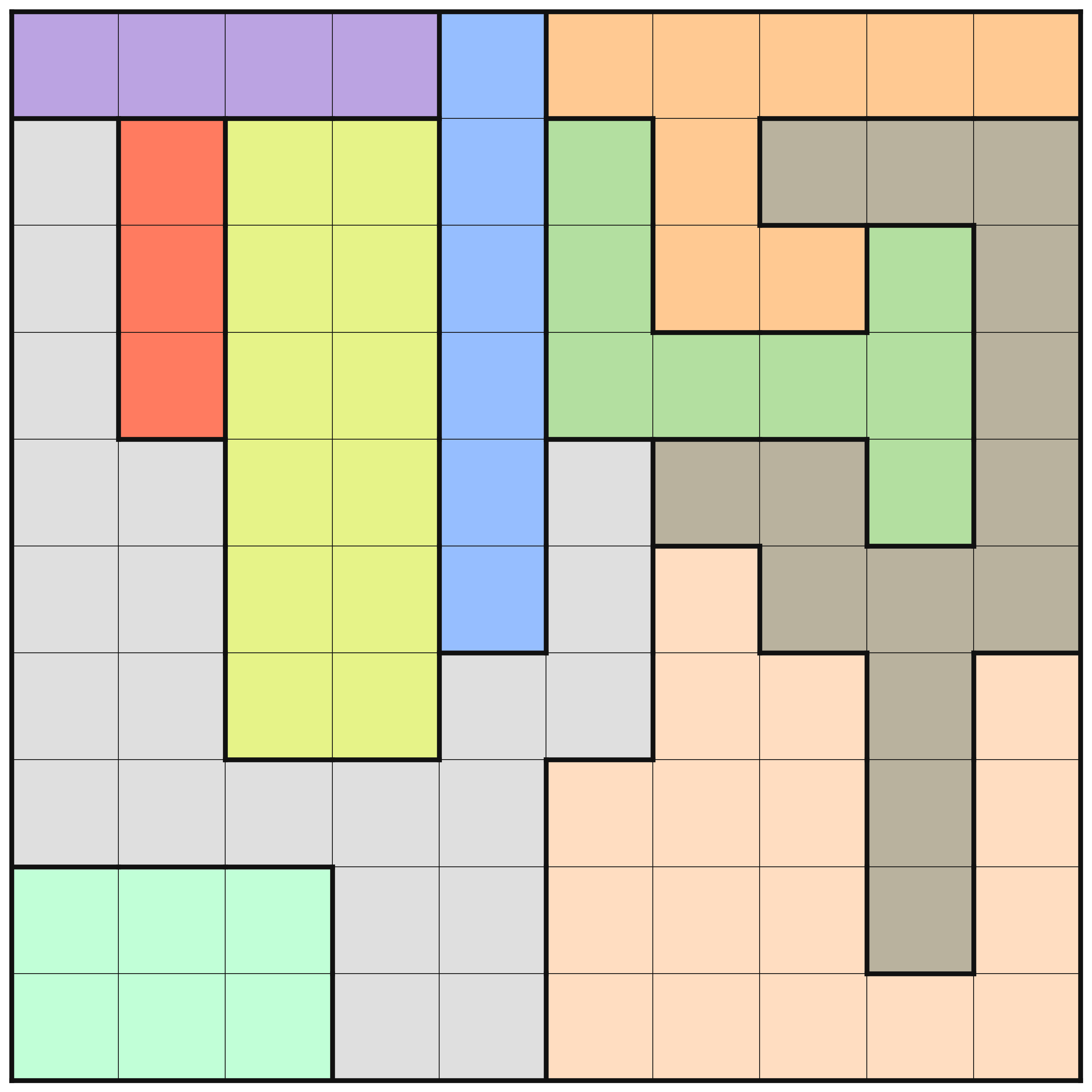
This puzzle instance is one of the more challenging ones. There are interesting differences in the amount of deductions that are made at the different optimization levels. At levels O0 to O2, no deduction is made from the MiniZinc pre-processing, but on levels O3, O4, and O5 there are. In the below images, the results for these three levels are shown. A cross in a square means that pre-processing has deduced that no queen can be placed in that square. A queen, naturally, means that pre-processing determined that that is where the queen should be.
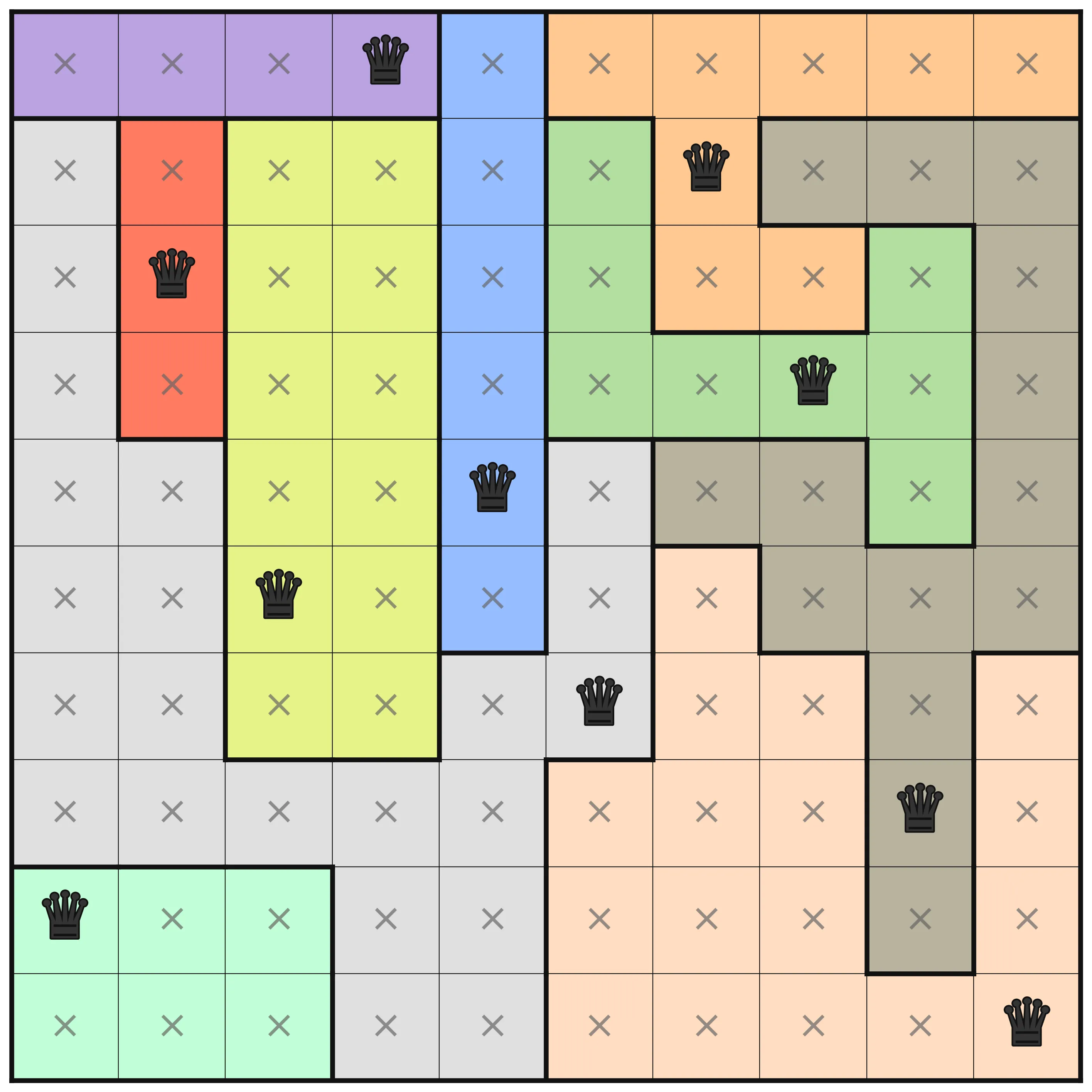
At the first level where pre-processing has happened (O3), the only thing is that the first row is marked so that the queen must be in the Purple area. The same analysis is not done for the symmetrical Red area, and that is because the choice of viewpoint makes a difference in how rows and columns are handled. A dual model that includes both row variables and column variables and links them using channeling constraints would have better initial propagation, but would not be significantly better in general.
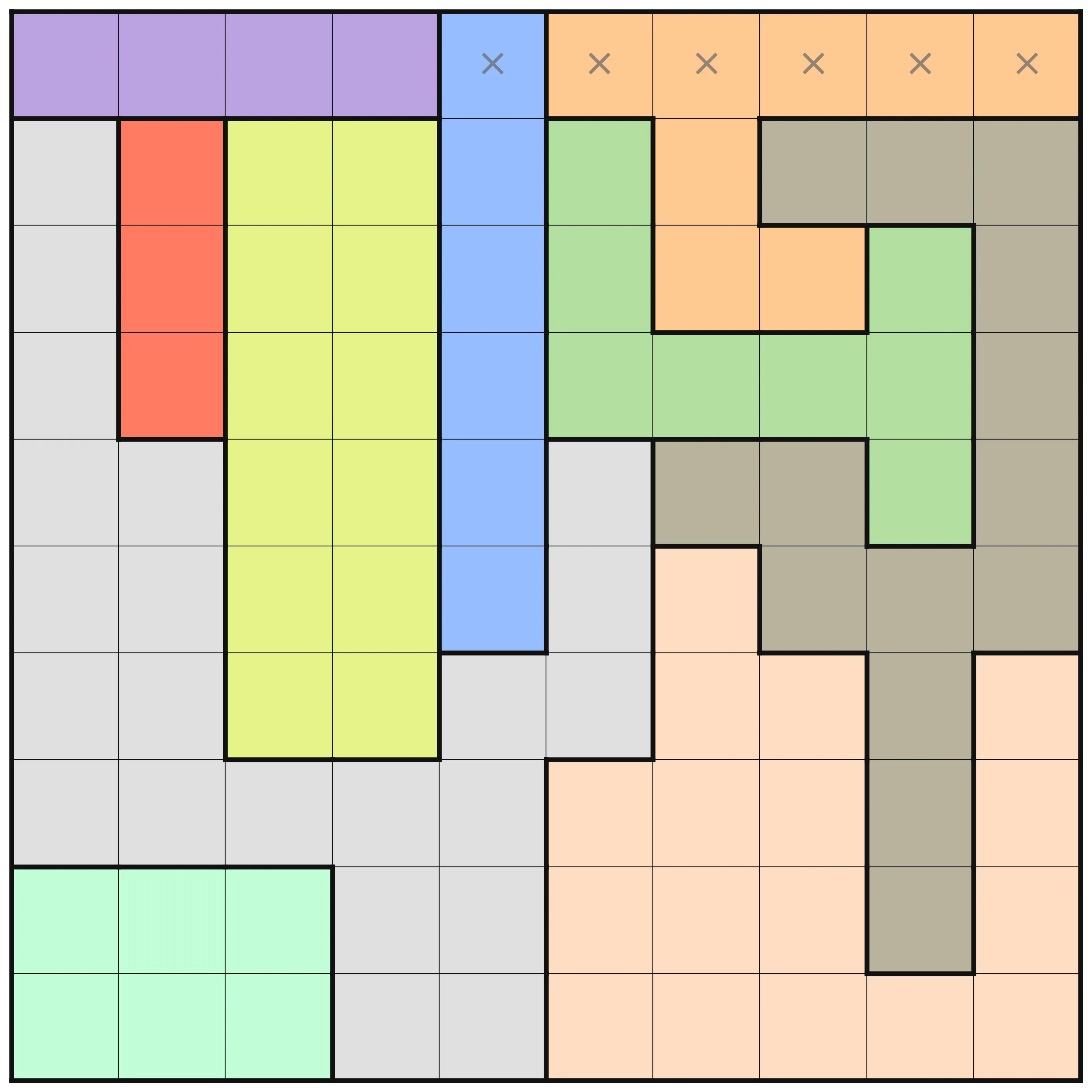
At O4 (the middle image), a lot more deductions have been made. For each row, the bounds of each variable (which column to place the queen in that row) have been adjusted using bounds shaving. For example, in the third row, assigning a queen to the first column (the lilac area) would remove any possibility to place in the red area. The resulting failure means that the bounds are adjusted. After all that, further propagation is done to make new deductions from all the new information.
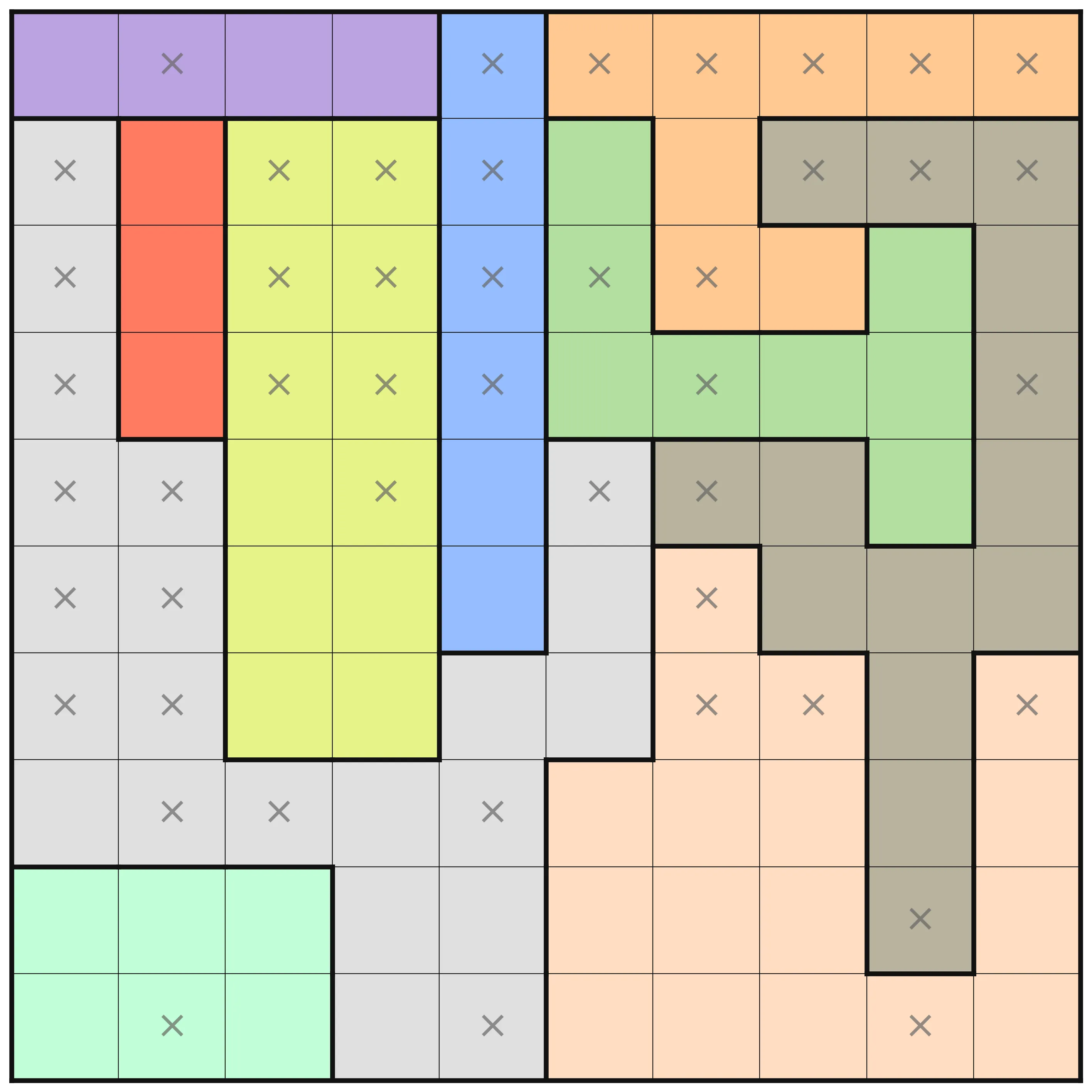
Finally, with domain shaving the puzzle is solved fully, before any search is done. Solving during pre-processing can be a great thing, but it comes at a cost in general.
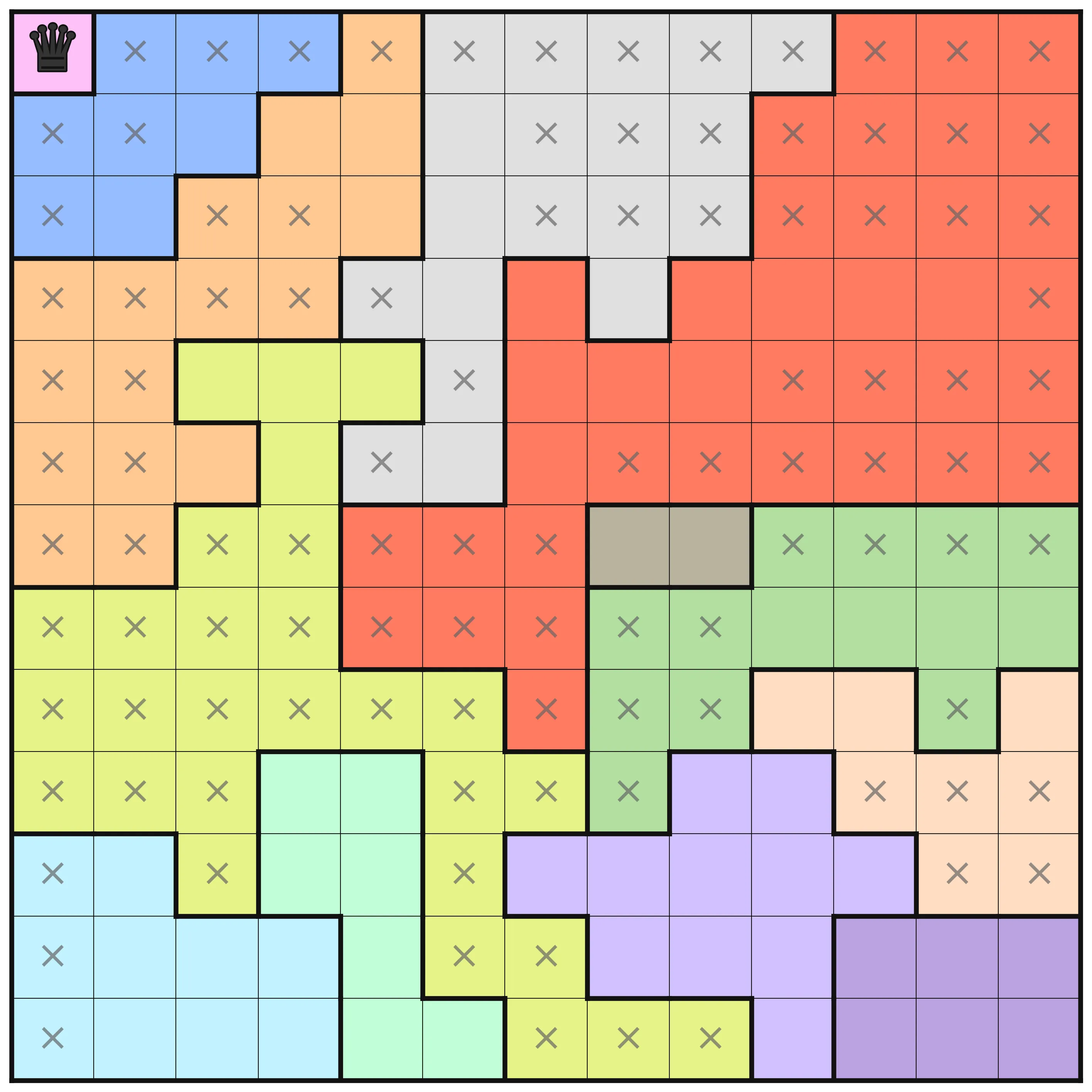
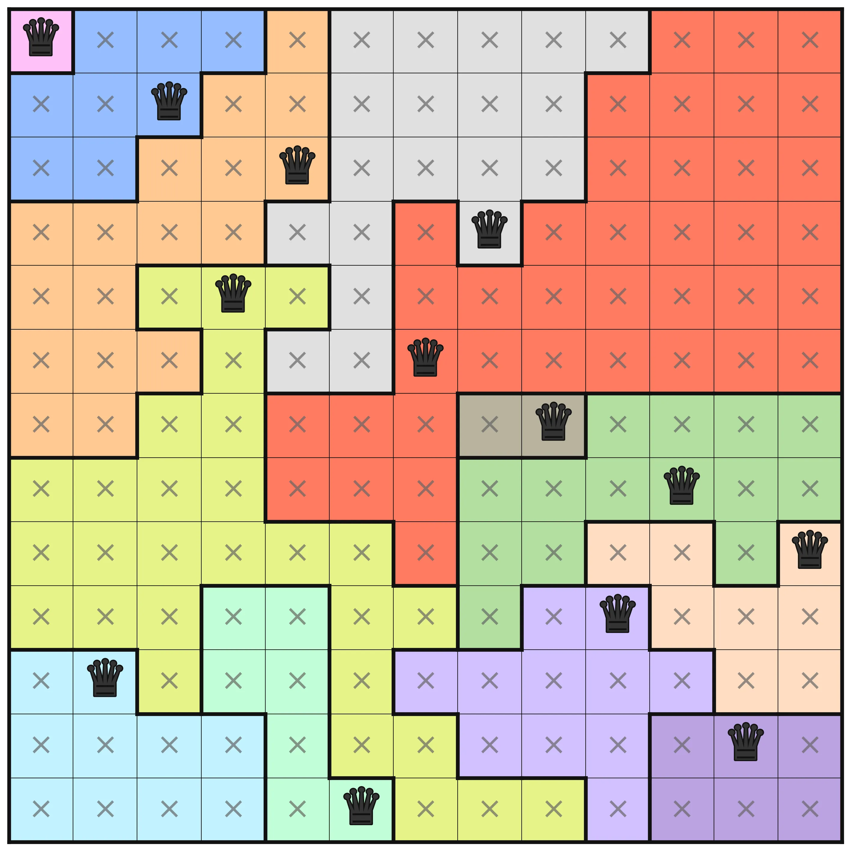
As another example, there is a 13 by 13 community level (level 195) that has similar change in the level of information gained at different optimization levels.
n = 13;
Colors = {A, B, C, D, E, F, G, H, I, J, K, L, M};
board = [|L, B, B, B, C, D, D, D, D, D, E, E, E |B, B, B, C, C, D, D, D, D, E, E, E, E |B, B, C, C, C, D, D, D, D, E, E, E, E |C, C, C, C, D, D, E, D, E, E, E, E, E |C, C, F, F, F, D, E, E, E, E, E, E, E |C, C, C, F, D, D, E, E, E, E, E, E, E |C, C, F, F, E, E, E, H, H, G, G, G, G |F, F, F, F, E, E, E, G, G, G, G, G, G |F, F, F, F, F, F, E, G, G, I, I, G, I |F, F, F, J, J, F, F, G, K, K, I, I, I |M, M, F, J, J, F, K, K, K, K, K, I, I |M, M, M, M, J, F, F, K, K, K, A, A, A |M, M, M, M, J, J, F, F, F, K, A, A, A ||];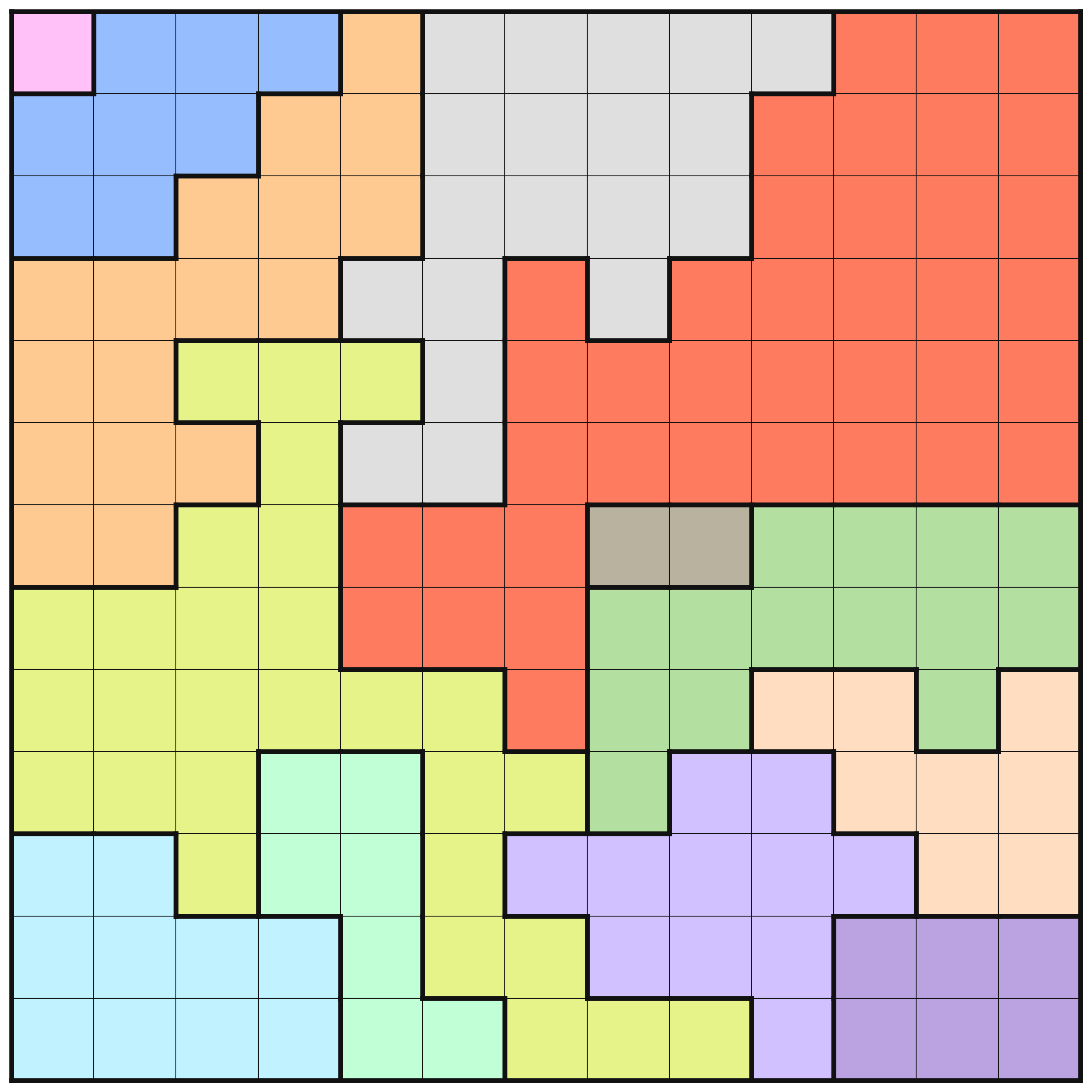
This puzzle has the following information at optimization levels O3, O4, and O5 respectively.

Measuring performance of combinatorial solvers and cactus plots 🌵
Combinatorial solvers try to solve NP-complete problems, and as we strongly suspect that , there is no silver bullet solution that will always work. This also means that for any type of system, the performance will have inherent variability.
A common way to measure performance for solving satisfaction problems is to run the systems on a large set of instances and to plot in a so-called cactus plot. The run-times for each solver tested are sorted, and a cumulative sum is computed. Plotting this cumulative sum (usually using logarithmic time) will show that if we run for a certain amount of time, we can at best solve this many problems.
Cactus plots are popular in the SAT community, where satisfiability questions are most common. For optimization problems where different solvers will find different solutions, there are other types of plots and measurements that can be used. One interesting such case is the method used in the MiniZinc Challenge. The method is further described in the paper Philosophy of the MiniZinc challenge by Stuckey, Beckett, and Fischer.
Solver configurations
We will test several different solvers in different configurations. The solvers tested are
- Gecode - a classical constraint programming solver
- Chuffed - a lazy clause generation solver
- OR-Tools CP-SAT - a portfolio lazy clause generation solver with a built-in MIP solver
- Pumpkin - a new lazy clause generation solver
- Huub - a new lazy clause generation solver
- HiGHS - a modern open source MIP solver
- COIN-OR CBC - a classical open source MIP solver
All solvers except Huub and Pumpkin are the versions bundled with MiniZinc 2.9.3.
Pumpkin is from the main branch at git sha d7e8bb02 from July 29th 2025.
Huub is from develop branch at git sha f41a98b from July 23rd 2025.
Both Pumpkin and Huub were compiled with cargo using Rust version 1.88.0.
For the Gecode, Chuffed, Pumpkin, and Huub solvers variants are tested searching for all solutions.
This mode will find out if the problem is well-formed or not, in that a valid puzzle should have a single solution only.
For the Gecode solver, there is also a variant that uses the domain consistent propagators for the all_different constraints,
and also variants using O5 minizinc pre-processing.
Summarizing, we are running these configurations
- Gecode (
gecode)- First solution
- First solution using O5 (
-O5) - All solutions (
-all) - With domain consistent propagation (
-domain) - With domain consistent propagation using O5 (
-domain-O5) - All solutions with domain consistent propagation (
-domain-all)
- Chuffed (
chuffed)- First solution
- All solutions (
-all)
- CP-SAT (
cp-sat)- First solution
- Pumpkin (
pumpkin)- First solution
- All solutions (
-all)
- Huub (
huub)- First solution
- All solutions (
-all)
- HiGHS (
highs)- First solution
- COIN-BC (
coin-bc)- First solution
Test instances
The test instances are collected from the repository queens-game-linkedin on GitHub.
The collection was done on August the 20th 2025, from the main branch at c836118.
In total, there are a almost 700 levels, with most of them being standard levels (469) that are taken from LinkedIn.
Out of the 689 total levels, 603 of them are well-formed with a single solution.
In the following benchmarks, only the well-formed puzzles will be used.
Unsuprisingly, the erroneous levels are from the community contributions and not from the levels published on LinkedIn.
| Category | Tested | Well-formed | Percentage |
|---|---|---|---|
| bonus-levels | 16 | 16 | 100.0% |
| community-levels | 204 | 118 | 57.8% |
| levels | 469 | 469 | 100.0% |
| Total | 689 | 603 | 87.5% |
The test instances also use different sizes, from 6 up to 11. In the below table, there is a breakdown of the sizes and their counts.
| Size | Tested | Well-formed | Percentage |
|---|---|---|---|
| 6 | 18 | 14 | 77.8% |
| 7 | 128 | 92 | 71.9% |
| 8 | 194 | 184 | 94.8% |
| 9 | 181 | 170 | 93.9% |
| 10 | 89 | 83 | 93.3% |
| 11 | 75 | 57 | 76.0% |
| 12 | 3 | 2 | 66.7% |
| 13 | 1 | 1 | 100.0% |
| Total | 689 | 603 | 87.5% |
Results
With all these preliminaries out of the way, now it is finally time to report on the results. All tests here are over the 603 instances in the test set that are well-formed.
Number of failures
First, let’s look at the distribution of failures. Here, we will only look at Gecode as it is a standard constraint programming solver. The first plot shows a histogram over the total number of failures to find all solutions using the standard model in Gecode. The plot uses a logarithmic scale for the number of instances in order to see the low values at all.
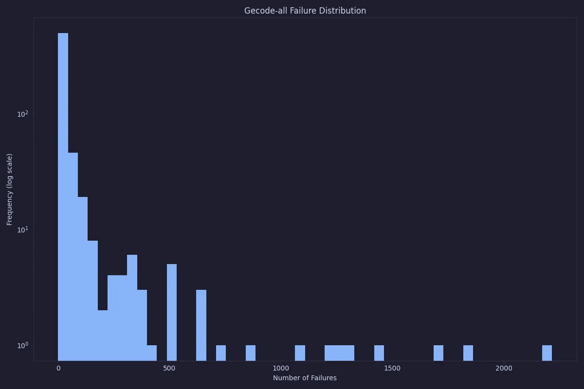
As can be seen, in almost all cases the number of failures is quite low, but sometimes it goes up to a couple of thousand nodes. This is still quite a low number of failures, and our expectation is that it will be quick to solve anyway. This can be compared with the number of failures when using O5 as pre-processing.
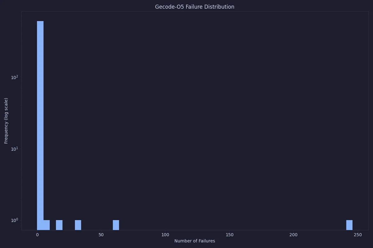
With O5, only three instances are not solved before search starts, which shows the potential of strong pre-processing. However, as we will see in the next section, this does not translate to faster overall total solve times.
The following table shows statistics for the number of failures for all the solvers that report this statistic.
Note that for a solver that is not marked with -all, the search may just be very lucky.
| Solver | Min | Max | Mean | Median | Std Dev | Zero Failures | Zero % |
|---|---|---|---|---|---|---|---|
| chuffed | 0 | 72 | 8.51 | 6 | 8.82 | 20 | 3.7% |
| chuffed-all | 1 | 156 | 15.64 | 11 | 16.53 | 0 | 0.0% |
| cp-sat | 0 | 10 | 0.02 | 0 | 0.43 | 542 | 99.8% |
| gecode | 0 | 1262 | 26.11 | 2 | 105.36 | 148 | 27.3% |
| gecode-O5 | 0 | 246 | 0.66 | 0 | 10.95 | 537 | 98.9% |
| gecode-all | 0 | 2216 | 54.05 | 7 | 195.71 | 87 | 16.0% |
| gecode-domain | 0 | 294 | 6.1 | 1 | 22.66 | 223 | 41.1% |
| gecode-domain-O5 | 0 | 73 | 0.22 | 0 | 3.34 | 537 | 98.9% |
| gecode-domain-all | 0 | 308 | 11.69 | 2 | 35.41 | 148 | 27.3% |
| huub | 0 | 395 | 17.7 | 8 | 34.62 | 26 | 4.8% |
| huub-all | 0 | 493 | 34.97 | 19 | 52.79 | 4 | 0.7% |
| pumpkin | 0 | 3133 | 74.06 | 15 | 239.84 | 24 | 4.4% |
| pumpkin-all | 0 | 4651 | 161.23 | 40 | 427.28 | 8 | 1.5% |
One interesting thing to note is the differences for Gecode between domain consistent and standard propagation. Using domain consistent propagation (without O5) increases the number of zero failures from 148 to 223. This shows that the increased propagation effort has a measurable impact on which problems are solvable.
Wall time cactus plots
Measuring timing for very short programs that may also include sources of randomness is hard. Normally, one would want to run each example multiple times, and make sure that the standard deviation for the run times is not too high. Here, we are mostly interested in trends. The somewhat large set of instances means that although any individual measurement may be messy, on average the trends will be stable. In addition, all the solvers are run interleaved, which means that any systematic slowdowns during execution from the environment will be mostly equal.
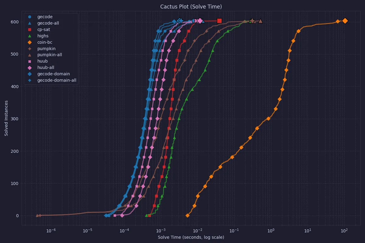
First, we will look at the wall time of running the whole MiniZinc system. This includes reading in the model and the problem instance, doing the required pre-processing, translating to FlatZinc, and then running the required solver on the FlatZinc.
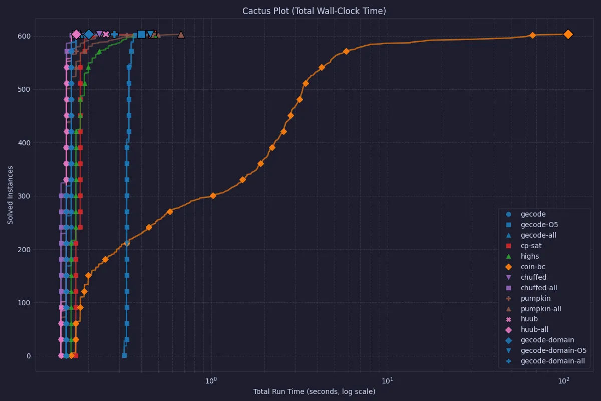
In the above plot, we can see that COIN-OR CBC is significantly slower than any other solver.
COIN-OR CBC is an older MIP solver, and may have troubles with the all_different constraints, as the linearization of that constraint is typically not that good.
Modern MIP solvers often have specialized systems to recognize and handle all_different-style models in order to overcome this.
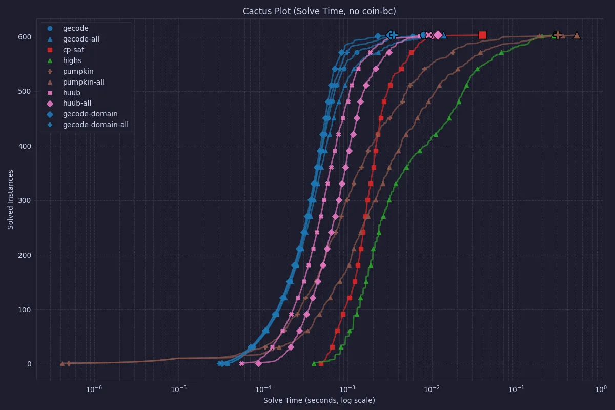
The differences between all other solvers are obscured by the outlier, so let’s look at the same data but without CBC.
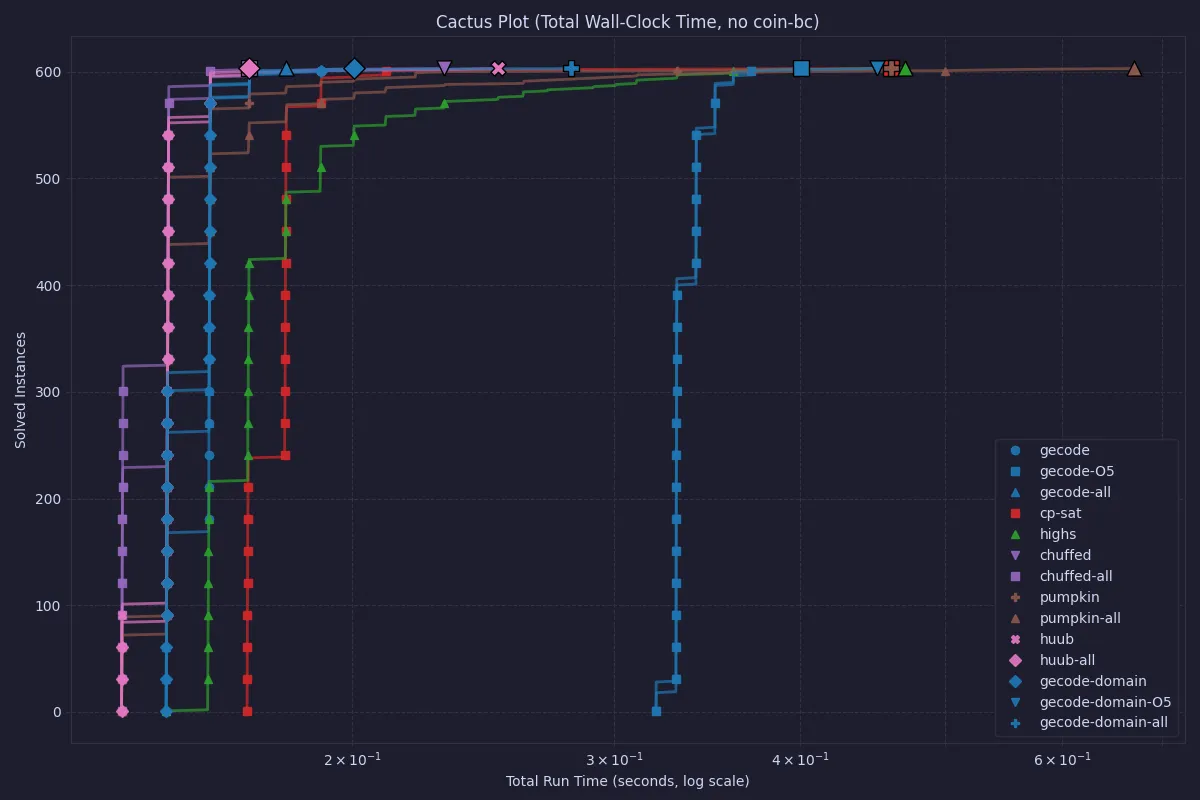
Here we can see that Chuffed and Huub are the overall fastest, and that using O5 processing (although it solved before search in most cases) does not in general lead to better solve times. Still, it is worth noting that the total times are quite small, so for any practical purposes, all solvers in this latter plot can be used.
It would definitely be interesting to see how the solvers would behave on larger instances.
Solve time
While the most interesting metric is the total wall clock time, some systems also report their solve time after reading the FlatZinc files. This can be interesting to indicate how a dedicated model in the used solver would behave if MiniZinc was not involved. Chuffed reports suspiciously odd times for this metric (almost always a 0), and so has been excluded from the graphs.
COIN-OR CBC is still the slowest when only looking at the solve time, so let’s also look at the same data without CBC.
For most of the instances, Gecode outperforms CP-SAT, but the end-points of the cactus plot are quite similar. For instances of this size, a dedicated model in either Gecode or CP-SAT would be very efficient.
Looking at the time it takes to solve a single problem for each solver, this box plot / violin plot shows the distribution of solve times.
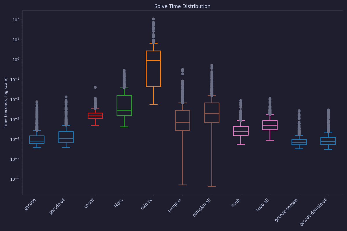
It is interesting to see that Pumpkin, while having a large variability, also has a lot of the fastest runs.
Solver choice
Given all the above results, what solver should one choose? The clearest indication is that the MIP solvers are less good at solving LinkedIn Queens. On the other hand, the actual differences in time between a modern MIP solver like HiGHS and either a classical CP solver like Gecode or an LCG solver like Chuffed or CP-SAT is small in absolute terms.
Summary
As mentioned in the beginning, the simple answer is that for simple problems like LinkedIn Queens, most methods work equally well. The main outlier is COIN-OR CBC which is an older MIP solver.
For a more meaningful comparison of solvers, it is much better to look at the MiniZinc Challenge. The results for the 2025 challenge were announced last week, and as usual Google OR-Tools won all the medals. It is worth looking at the detailed results though, as there are many solvers that are entered by the organizers that are not eligible for medals. In addition, it is not the case that OR-Tools CP-SAT is the best for every problem, so while it is a very good allround solver it is not always the right choice.
Footnotes
-
Adding a propagation annotation such as
domain_propagationis a request, as it is not a requirement that the solver must follow the annotation.In particular, the solver might not even implement the constraint as a propagator where this request would make sense. Consider a MIP solver such as HiGHS shown above, where all the constraints are simple linear relations. ↩