Planning with open variable lists in GecodeDRAFT
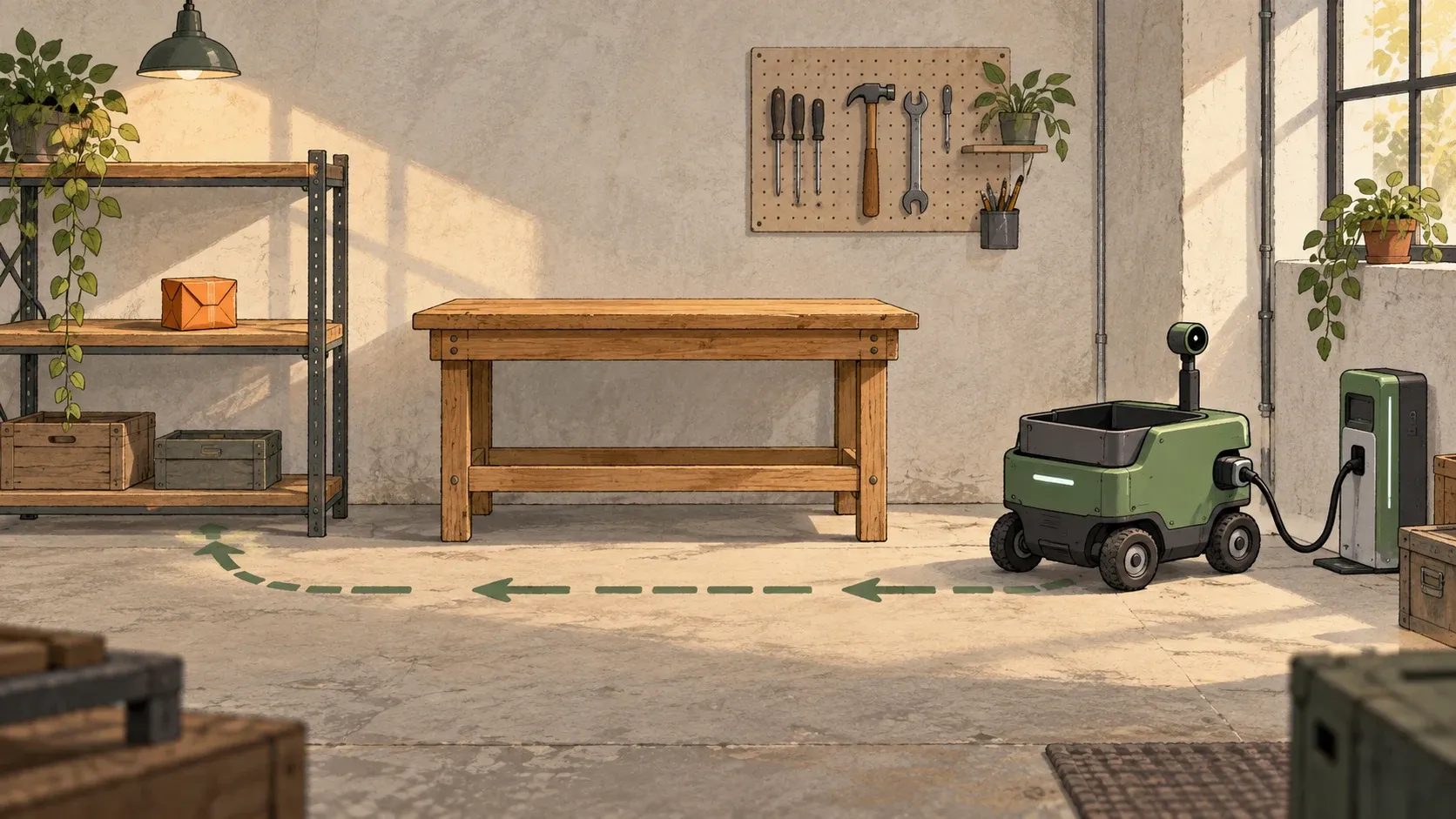
A robot needs to fetch a packet from the shelf and put it down on the workbench. Easy enough: drive over to the shelf, pick up the packet, drive back, and put it down. Four actions. Unless the battery is low. Then the robot has to visit the charger first, and the questions become where in the plan that visit should go, and how long the robot should stay there.
This is planning in miniature: a start, some actions, a goal, and nobody telling us how long the plan should be.
Planning is a research field of its own, and a common first idea is to describe the problem in PDDL and hand it to one of the many planning systems that read it. For a lot of problems, that is the right choice. Constraint programming is another natural fit, especially when the actions come with restrictions like a battery that runs down. The common objection is that most constraint programming solvers fix the set of variables before search starts, so we need a bound on the length of the plan before we know how long it will be.
Gecode has always allowed new variables and constraints to be added during search, but before Gecode 6.5.0 there was no explicit support for it.
Gecode 6.5.0 adds that support as open variable lists.
An OpenIntVarList is a list of ordinary IntVars that are created when propagation or search needs another position, together with an ordinary IntVar for its length.
When a position is added, a transition callback can create more variables and post constraints for that step, such as the next state of a plan, so any constraint in Gecode can be used in a model that grows.
In addition, the release has open versions of some common constraints, such as regular, distinct, and sequence, which are posted once on the whole list and follow it as it grows.
A list brancher decides both the next value and whether the list should grow, and most of the usual variable and value selectors work on the positions.1
All of this is built with the propagator and brancher interfaces that Gecode already had, plus a few small additions to the kernel.2
The release also includes two experimental search engines, A* and complete anytime beam search. This post models the robot, then the fifteen-puzzle, and ends with the new engines.
A delivery with a charging detour
The shelf, the workbench, and the charger are connected in a line, in that order, as in the picture at the top. The robot starts at the workbench with one unit of charge. Each move uses one unit, each charge action at the charger adds one, and the battery holds five. Picking up and putting down the packet are free.
With one unit, the robot can reach the shelf, but then it is stuck there with the packet. The shortest working plan visits the charger first.
| Action | Location afterwards | Charge remaining | Packet |
|---|---|---|---|
| Initial state | Workbench | 1 | On the shelf |
| Move to charger | Charger | 0 | On the shelf |
| Charge | Charger | 1 | On the shelf |
| Charge | Charger | 2 | On the shelf |
| Charge | Charger | 3 | On the shelf |
| Move to workbench | Workbench | 2 | On the shelf |
| Move to shelf | Shelf | 1 | On the shelf |
| Pick up | Shelf | 1 | Carried by the robot |
| Move to workbench | Workbench | 0 | Carried by the robot |
| Deliver | Workbench | 0 | Delivered |
Three charges are exactly enough, and with two the robot is stuck at the shelf. Charging four or five times also works, but every extra charge makes the plan longer, so the first plan a solver finds need not be the shortest. Try it below, and head straight for the shelf first to see what happens.
Workshop planning
Each move uses one unit of charge.
Manual controls
Follow the plan
Step 0 of 9Optimal plan: Right → Charge → Charge → Charge → Left → Left → Take packet → Right → Deposit packet
What I want is a model that just describes the actions and their effects, and lets the solver discover the detour on its own.
How many actions should the model contain?
A straightforward CP model has a variable for each action, variables for the state before and after each action, and a transition constraint relating them. For a plan with four actions, there are four action variables and five states, with the first state fixed to the initial situation and the last required to satisfy the goal. For our example, that model has no solution. Planning encodings have traditionally dealt with the unknown length in two ways. One is to solve again with five actions, then six, and so on up to nine, so that the first plan found is also a shortest one. The other is to choose an upper bound, say twelve actions, and allow an unused suffix, at the price of modelling which positions are active and having every position up to the bound in the model from the start.
An open list gives a third option: keep the bound of twelve, but create positions only when search or propagation needs them. The model then grows the way a plan does when you work it out by hand: first the charging visit, then the trip to the shelf, and once the packet is delivered, we can stop.
A plan that grows
The full model is in open-robot.cpp. The actions are kept in an open list, and the states between them in three more: where the robot is, how much charge it has, and where the packet is.
class Delivery : public IntMinimizeScript { OpenIntVarList actions, at, charge, packet;public: Delivery(const DeliveryOptions& opt) : IntMinimizeScript(opt), actions(*this, IntSet(ToShelf, Charge), [](Space& home, OpenIntVarList, int i) { static_cast<Delivery&>(home).step(i); }, opt.limit()), at(*this, IntSet(Shelf, Charger), opt.limit()+1), charge(*this, IntSet(0, capacity), opt.limit()+1), packet(*this, IntSet(OnShelf, Delivered), opt.limit()+1) { rel(*this, at.length() == actions.length() + 1); rel(*this, charge.length() == actions.length() + 1); rel(*this, packet.length() == actions.length() + 1); rel(*this, at.get(*this, 0), IRT_EQ, Workbench); rel(*this, charge.get(*this, 0), IRT_EQ, opt.charge()); rel(*this, packet.get(*this, 0), IRT_EQ, OnShelf); post_goal(*this, packet[0], actions.length(), 0); }Each action is an IntVar over the six action codes, and there are at most twelve of them.
actions.length() is the length of the finished plan, and actions.known_length() counts the positions created so far.
Creating a position is called materialization, and it does not assign a value.
When the plan grows, the new action is materialized and the callback calls step, which materializes the state after it and posts the constraints between them.
void step(int i) { at.materialize(*this, i+2); charge.materialize(*this, i+2); packet.materialize(*this, i+2); if (failed()) return; post_step(*this, actions[i], at[i], charge[i], packet[i], at[i+1], charge[i+1], packet[i+1]); post_goal(*this, packet[i+1], actions.length(), i+1);}The callback is shared between copies of the space, so it casts the space it is given instead of capturing this.
It must also be deterministic, since recomputation and parallel search may repeat an extension in another space.
The legal steps are a table with one tuple for each action and the states before and after it, posted as an extensional constraint for each step.
static TupleSetrobot_steps(void) {  TupleSet t(7);  // Moving to a neighbouring location uses one unit of charge. A move  // action has the same code as its destination.  for (int pk=OnShelf; pk<=Carried; pk++)    for (int ch=1; ch<=capacity; ch++)      for (int at=Shelf; at<Charger; at++) {        t.add({at+1, at, ch, pk, at+1, ch-1, pk});        t.add({at, at+1, ch, pk, at, ch-1, pk});      }  // Charging adds one unit, up to the capacity.  for (int pk=OnShelf; pk<=Carried; pk++)    for (int ch=0; ch<capacity; ch++)      t.add({Charge, Charger, ch, pk, Charger, ch+1, pk});  // The packet is picked up at the shelf and delivered at the workbench.  for (int ch=0; ch<=capacity; ch++) {    t.add({PickUp, Shelf, ch, OnShelf, Shelf, ch, Carried});    t.add({Deliver, Workbench, ch, Carried, Workbench, ch, Delivered});  }  t.finalize();  return t;}
static voidpost_step(Home home, IntVar a,          IntVar at0, IntVar ch0, IntVar pk0,          IntVar at1, IntVar ch1, IntVar pk1) {  static const TupleSet steps = robot_steps();  extensional(home, IntVarArgs({a, at0, ch0, pk0, at1, ch1, pk1}), steps);}
The goal decides where the plan ends.
static voidpost_goal(Home home, IntVar pk, IntVar length, int i) { BoolVar done = expr(home, pk == Delivered); rel(home, (length == i) >> done); rel(home, done >> (length <= i));}The plan can only end where the packet has been delivered, and it ends as soon as it has.
Propagation does some planning before search starts. The packet cannot be delivered in fewer than four actions, so the root already has four, the first a move to the shelf or the charger and the second picking up or charging. Branch-and-bound then finds the nine-action plan.
Actions: 9 to-charger charge charge charge to-workbench to-shelf pick-up to-workbench deliverThe same transitions as an automaton
We can also use the regular constraint to encode the state as a transition system, folding the values of at, charge, and packet into the states of a finite automaton instead of keeping them in variables.
Each tuple in the table becomes a transition labelled with its action, so the accepted words are exactly the delivery plans.
static intstate(int at, int ch, int pk) {  return (pk * (capacity+1) + ch) * 3 + at;}
// Read the table of steps as an automaton over the actions.static DFArobot_dfa(int initial_charge) {  TupleSet steps = robot_steps();  std::vector<DFA::Transition> transitions;  for (int i=0; i<steps.tuples(); i++) {    // A step is (a, at0, ch0, pk0, at1, ch1, pk1).    TupleSet::Tuple s = steps[i];    int action = s[0];    int from = state(s[1], s[2], s[3]);    int to = state(s[4], s[5], s[6]);    transitions.push_back({from, action, to});  }  transitions.push_back({-1, 0, 0});  // The plans end in the states where the packet has been delivered.  IntArgs delivered;  for (int ch=0; ch<=capacity; ch++)    for (int at=Shelf; at<=Charger; at++)      delivered << state(at, ch, Delivered);  delivered << -1;  int start = state(Workbench, initial_charge, OnShelf);  return DFA(start, transitions.data(), delivered.begin());}
The model is then just the action list and one constraint, with no state lists and no callback.
extensional(*this, actions, robot_dfa(opt.charge()));The interesting part is what an open regular constraint does with an unfinished plan. After moving to the charger and charging once, the packet is still on the shelf, but the plan can still reach the goal. Moving straight to the shelf is a dead end, and is rejected while the list is still open. So while the list is open, a prefix is kept if it can reach an accepting state within the maximum length, and once it is closed, its last state must be accepting.
Regular propagation works on a layered graph, with a layer of automaton states for each position and edges labelled with the values in each domain.
The widget uses a small automaton for the words that start with a and end with b.
With a fixed length of two, only ab has a path.
The open list has the same two positions but a length of up to four, so a prefix like aa can still become aab.
Lower the maximum length to two, and the open list behaves like the fixed one.
A DFA and its unfoldings
The DFA
Fixed-length unfolding
length = 2Open list and possible continuations
2 ≤ length ≤ 4Open, so a prefix ending in q₁ can still finish with b.
Gecode does not build the future layers.
It computes the shortest distance from each automaton state to an accepting state, and keeps an end state of the prefix only if that distance fits within length().max() - known_length().
Both the table and the automaton list every combination of location, charge, and packet status. That works for the robot, but with more packets and a second robot the combined states explode, and the transitions are better posted as ordinary constraints over the state variables, as in the fifteen-puzzle below.
Searching over actions and length
The list brancher assigns the materialized positions, and once they all have values, it tries closing the list, with extending it as the alternative. For the robot, closing fails until the packet is delivered.
branch(*this, actions);The usual selectors choose among the materialized positions. To settle the number of actions first, branch on the length before the actions, and depth-first search with minimum-value selection then tries shorter plans first.
branch(*this, actions.length(), INT_VAL_MIN());branch(*this, actions, INT_VAR_SIZE_MIN(), INT_VAL_MIN());Building the plan incrementally can find a longer plan before a shorter one, so the companion minimizes the length with branch-and-bound.
With -branching max, it tries the highest action code first, which means charging whenever it can, and finds plans of eleven, ten, and finally nine actions.
Constraints over a growing plan
Real planning models collect side rules: don’t repeat an action, don’t keep the charger busy too long, pick up before you deliver. The open constraints in the release express rules like these, posted once and applied to every new position.
rel(*this, actions, IRT_NQ); // no immediate repeatssequence(*this, actions, IntSet(Charge, Charge), 4, 0, 3); // at most 3 charges in 4precede(*this, actions, PickUp, Deliver); // pick up before deliveringdistinct(*this, jobs); // each job at most oncesliding_sum(*this, loads, 4, 0, 6); // load in each window of 4min(*this, levels, lowest); // lowest battery levelThe last three assume other open lists, of jobs, loads, and battery levels. Side rules can change which plans exist at all. For the robot, forbidding immediate repeats leaves no plan, since a single charge never pays for the trip there and back, while at most three charges in every window of four removes the two longer plans and keeps the nine-action one.
What makes these constraints different from their closed versions is the positions that do not exist yet.
sequence and sliding_sum only count complete windows, so a plan shorter than the window is unrestricted.
distinct remembers the assigned values and removes them from positions created later.
min and max can only bound the result from one side while the list is open, since a later position can still lower the minimum or raise the maximum.
Solving the classic fifteen-puzzle
The fifteen-puzzle is the classic test problem for heuristic search, with far too many boards for a table or an automaton. Fifteen numbered tiles and a blank occupy a four-by-four board, and a move slides a tile next to the blank into the blank. The goal has the tiles in order, with the blank at the bottom right. This board needs two moves: slide tile 14 left, and then tile 15.
Click a tile beside the blank to slide it. With the board focused, arrow keys move the blank.
Seen from the blank, it moves right twice, so a plan can be described by the successive positions of the blank.
Gecode’s fifteen-puzzle.cpp uses two open lists: path[i] is the cell of the blank in board i, and the sixteen entries from tiles[16*i] are board i, with 0 for the blank.
Only path has a transition callback, which creates the board for each new blank position.
tiles(*this,IntSet(0,15),16*(opt.limit()+1)),path(*this,IntSet(0,15), [](Space& home, OpenIntVarList x, int i) { static_cast<OpenPuzzle&>(home).transition(x,i); },opt.limit()+1)The constructor body ties the two lengths together, fixes the first board, and bounds the length from below.
rel(*this,tiles.length() == 16*path.length());IntVar start = path.get(*this,0);post_start(*this,state(0),start,initial);rel(*this,path.length() >= manhattan(initial)+1);The Manhattan distance, the sum of each tile’s distance to its goal cell, is a lower bound on the number of moves, so propagation creates several boards before any move is chosen.
Each new blank position materializes its board, connects it to the previous one, and posts the goal, just like the robot’s step.
voidtransition(OpenIntVarList x, int i) { tiles.materialize(*this,16*(i+1)); if (failed()) return; if (i > 0) post_slide(*this,state(i-1),x[i-1],state(i),x[i]); post_goal(*this,state(i),path.length(),i+1);}A slide moves the blank to a neighbouring cell, puts the moved tile in the old blank cell, and leaves every other cell unchanged.
extensional(home,IntVarArgs({old_blank,new_blank}),adjacent);rel(home,element(after,old_blank) == element(before,new_blank));rel(home,element(after,new_blank) == 0);for (int i=0; i<16; i++) { rel(home,((old_blank != i) && (new_blank != i)) >> (before[i] == after[i]));}Every board is a permutation of the tiles, so an assigned path determines all the boards, and it is enough to branch on path.
The example also has a fixed model, -model fixed, that creates every board up to the move limit and uses a branch filter so that search does not choose moves after the goal.
For a two-move solution with a limit of eight, it has nine boards where the open model has three.
build/bin/fifteen-puzzle -model open -search bab -branching min \ -scramble 4 -limit 8 -seed 1 -solutions 0This finds plans of eight, six, and finally four moves, which matches the initial Manhattan distance, and -model fixed finds the same optimum.
Heuristic search for planning
Gecode 6.5.0 also includes two experimental search engines, AStar and CABS (complete anytime beam search), enabled with GECODE_ENABLE_EXPERIMENTAL=ON in CMake or --enable-experimental with Autoconf.
They work with any Gecode space, with or without open lists, and their APIs may still change.
Branch-and-bound explores depth-first, and has no idea which of the pending partial plans looks most promising. Heuristic search estimates how good the best completion of each partial plan can be, and explores the most promising ones first. It is also the workhorse behind many of the planning systems mentioned at the start. The estimate must be admissible, never above the true cost. For the robot, ignoring the battery gives one: after moving to the charger and charging once, two actions are used and at least five remain, a bound of seven where the true total is nine.
Both engines take a Search::HeuristicGuidance, whose bound callback returns an optimistic value for the total objective, including the cost so far, and must be exact on solutions.
For the puzzle, the bound is the number of moves made so far plus the Manhattan distance of the board they lead to.
intdepth(void) const {  int i = 0;  while (i+1 < path.known_length() && path[i+1].assigned())    i++;  return i;}
intbound(void) const {  const int g = depth();  const int h = manhattan(values(state(g)));  return std::max(g+h,path.length().min()-1);}
depth stops at the first undecided move, even when later boards have been created, and the length gives the bound instead when it is stronger.
Search::HeuristicGuidance guidance(Search::HeuristicGuidance::MINIMIZE, [](const Space& home) -> std::int64_t { return static_cast<const Model&>(home).bound(); });opt.guidance(&guidance);if (opt.search() == PuzzleOptions::SEARCH_ASTAR) Script::run<Model,AStar,PuzzleOptions>(opt);else Script::run<Model,CABS,PuzzleOptions>(opt);Both engines use the model’s constrain to require improvement after each solution, so as with branch-and-bound, the first solution need not be optimal.
A* keeps every pending state.
CABS keeps only a beam of candidates at each layer of the search tree, starting with a width of one and doubling it while the discarded candidates might still lead to a better solution.
That finds a plan quickly, and spends more effort later on improving it and proving optimality.
CABS can also use a dominance test, which discards a candidate when another one can match each of its completions with one that is no worse.
Gecode’s tsptw.cpp, for the travelling salesman problem with time windows, offers all three engines on a closed model. I wrote an open-list variant that creates each position of the tour when the tour reaches it. Every tour visits all customers, so stating its length would create every position at the root. Instead, the variant states the goal as a condition on the visited customers.
BoolVar last = expr(*this, x.length() == i+1);IntVarArgs prefix(i+1);for (int j=0; j<=i; j++) prefix[j] = x[j];for (int k=1; k<p.n; k++) member(*this, prefix, IntVar(*this,k,k), imp(last));Both models find and prove the optimal travel times for the two built-in instances with branch-and-bound, A*, and CABS. The instances are far too small to say which combination works best on hard problems.
When to use an open plan
Leaving future positions uncreated is a tradeoff. They take no storage, but their domains are not available for propagation either, so a fixed-horizon model may detect some failures earlier. My guess is that open lists pay off when a large upper bound is needed to admit all plans, while most of the search works with much shorter prefixes, but that needs measuring. For classical planning problems, a dedicated planner will often be the better tool. A constraint model becomes interesting when the plan also has to satisfy side constraints, like resource limits, time windows, or the rules above.
Back in the workshop, the model is the same whatever the initial charge. With a full battery, the shortest plan is the direct four actions, and with a single unit, it is the nine-action detour. Nobody had to guess the length of the plan in advance. The model describes what the robot can do, and search works out how long it takes.
Footnotes
-
The exceptions are the activity-based (Action) and conflict-history (CHB) variable selectors. They require the complete list to be materialized when the brancher is posted, so they cannot be used for positions created later. ↩
-
For example, callbacks run inside a
Space::NoGPIscope, so that propagators created and discarded during search do not accumulate global propagator information such as the accumulated failure count (AFC). A callback can open aSpace::UseGPIscope for postings that should be tracked as usual. ↩