Writing a custom propagator is worth considering when one constraint carries much of a problem’s structure. My paper Propagation Algorithms for the Minimum-Distance Constraint over Selected Points, to be presented at ModRef 2026, works through one such case in Gecode.

Suppose we want to select five facility locations, spread out so that the closest pair is as far apart as possible. Let z denote that minimum distance. A straightforward CP model introduces a distance variable for every selected pair, then constrains z to be the minimum of those distances. This is a clear specification, but it creates quadratically many auxiliary variables and propagators.

I implemented several ways for Gecode to handle that relation directly: small pairwise propagators, global support scans, advisor-backed versions that remember which pairs need to be revisited, and an upper bound based on matchings in a conflict graph.

A small instance#

Consider the eight candidate sites below. We must choose five. The highlighted selection {A, C, E, F, G} has minimum distance 4, attained by F and G.

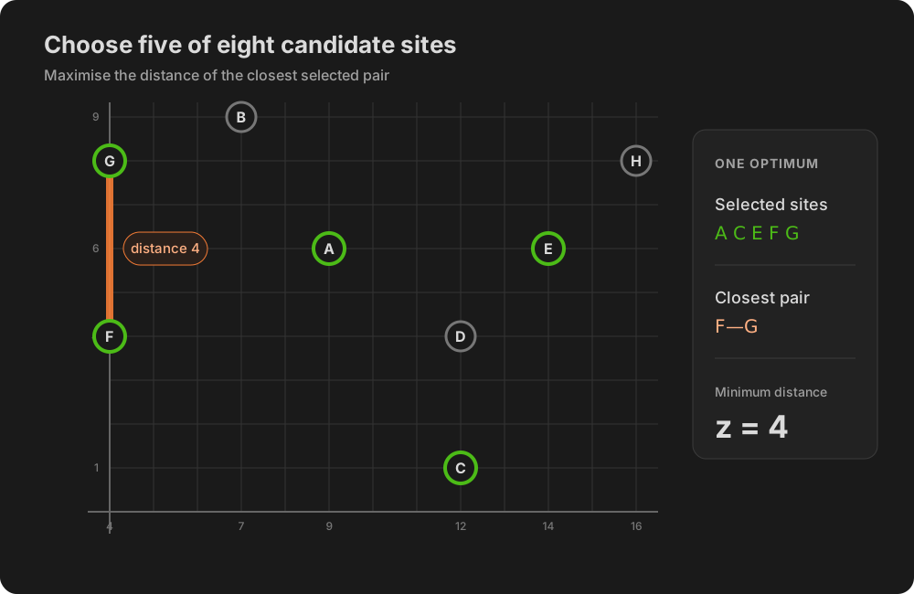
That gives us a lower bound of 4. The next larger pair-distance level in this instance is 5, so proving optimality amounts to ruling out every selection whose minimum distance is at least 5. We will return to that after introducing the propagators.

Propagator variants#

The variants differ in both the inference they perform and how they organise the work.

The advisor-backed rows in the results therefore change how work is scheduled and remembered, while the matching suffix adds another upper-bound argument.

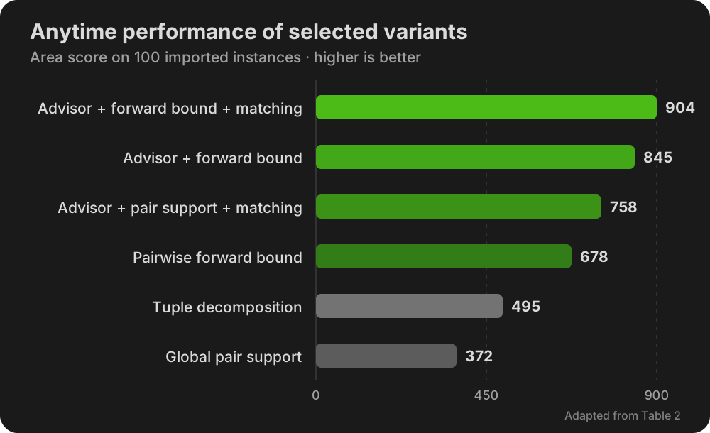
The figure adapts the main experimental table from the paper. The 100 imported p-dispersion instances all ask the solver to select well-spaced points. The MiniZinc Challenge area score rewards variants that find useful solutions early and continue improving them; higher is better. In these tests, the advisor-backed forward-bound propagator with the matching bound performs best. The simpler pairwise forward-bound propagator remains competitive, while the global pair-support scan scores below the tuple decomposition in this comparison.

How the greedy maximal matching bound works#

Take a candidate threshold t. Let the active sites be the union of the current selected-position domains. Build a conflict graph on those sites, with an edge between two sites when their distance is strictly less than t. A selection with minimum distance at least t must be an independent set in this graph. The propagator then computes a greedy maximal matching in the conflict graph.

Any matching gives a sound upper bound on the size of such an independent set; the propagator builds one greedily until it is maximal. Each matching edge has disjoint endpoints, and an independent set can contain at most one endpoint from each edge. If the active graph has n vertices and the matching has m edges, then the largest independent set, written α(Gₜ), satisfies

α(Gₜ) ≤ n − m.

Now return to the eight-site instance. At threshold 5, the conflict edges are AB, AD, BG, CD, DE, EH, and FG. The four highlighted edges below form one greedy maximal matching: AB, CD, EH, and FG.

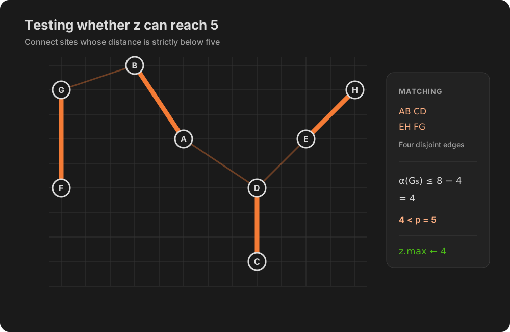
The matching proves that an independent set contains at most 8 − 4 = 4 sites. We need five, so a minimum distance of 5 is impossible and the propagator can lower z.max to the preceding distance level, 4. The selection in the first figure attains 4, so the lower and upper bounds meet: its minimum distance is optimal.

This is only an upper-bound certificate. A greedy maximal matching may fail to find a certificate even when the threshold is impossible, and passing the test does not prove that the threshold is feasible. Different maximal matchings can also have different sizes, so propagation may depend on which edges the greedy algorithm encounters first.¹ The strict conflict test matters as well: points exactly 4 apart, such as F and G, remain compatible when testing t = 4.

Writing the custom constraint paid off here: it avoids auxiliary distance variables, advisors remember which pairs changed, and the matching pass adds a problem-specific upper-bound certificate. The advisor-backed forward-bound variant with matching has the best anytime score in this comparison, while the simpler pairwise forward-bound propagator remains competitive and considerably easier to implement. The experiments are preliminary and do not identify a universally best implementation, but they show what becomes possible once the solver can see the problem’s structure. The details and complete comparison are in the paper.

Footnotes#

1. A maximum matching could strengthen the certificate by finding the largest possible m. The classical approach is Edmonds’ blossom algorithm, with complexity O(n²|E|) for n active sites and conflict-edge set E, compared with O(n²) for the simple greedy maximal matching used here. Blossom-style algorithms are also substantially harder to implement. Faster maximum-matching algorithms exist, but bring either more implementation complexity or significant constant factors. For this propagator, the greedy algorithm is a deliberate cost-strength tradeoff. ↩